Georgia institute of technology CSE-6242 Final Project
Buying vs Renting: A Data-Driven Housing Affordability Project
James Marvin | Michael Cheng | Qing Yu | Tyler Chang | November 22, 2024
0. Introduction
For many Americans, owning a home represents a key life milestone. Yet, in recent years, achieving homeownership has become significantly more difficult. As of Q3 2024, only one-third of U.S. households could afford a single-family home, a sharp decline from nearly two-thirds just five years earlier, driven by soaring home prices and nearly doubled mortgage rates [1]. This housing crisis is especially real in California, according to Norada Real Estate Investments, only 16% of households across California can afford a median home price at $1.2 million dollars, requiring a minimum annual income of $220,800 [2]. As a result, nearly half of all renter households spent more than 30% of their income on rent in 2021 [3].
1. Problem
Although housing affordability is a real issue for many Americans, there is no existing tooling today that provides enough information for people to understand whether renting or buying a home is a better option for them. Today, there are many online real estate platforms that buyers and renters use to search for potential homes. Although platforms like Zillow and Redfin do a good job at serving available listings to users, these tools do not make it easy for users to:
Locate areas where buying/renting is the more affordable option
Dynamically calculate a monthly payment based on different conditions (e.g. interest rates) and compares directly with rental data
Forecast a renter’s future rental costs and a home buyer’s projected home value (e.g. 5 years from now)
This type of information is crucial to an individual or family’s decision to buy or rent and is largely unavailable on all major real estate products. The goal of this project is to create a tool that helps demystify these 3 areas to help users make a data-informed decision when choosing to rent or buy.
2. Our Solution
Our Interactive Tableau Dashboard (Figure 1) surfaces available listings in the Bay Area where a user can: 1) understand where buying/renting is cheaper, 2) personalize their search to their specific needs or financial circumstance, and 3) observe a rental’s forecasted monthly cost or a property’s forecasted valuation in different time horizons.
3. Proposed Method
3.1 Intuition
The current literature looks to understand valuation of a home through general economic output or based on general amenities that are local to the area [4-5]. Aizenman, J.et al describe in their model that funding supply, credit conditions, and employment are key factors however they fail to look at inherent factors specific to the home [5]. Numan, Jamal A. A., and Izham Mohamad Yusoff in "Identifying the Current Status of Real Estate Appraisal Methods" looked at the current techniques used for housing valuation and found many of the machine learning models were based in countries outside of the US, with the majority being in China, which does not directly apply in our situation [6].
Our method factors in comprehensive homeowner and renter cost components (e.g., mortgage payments, property taxes, HOA fees, maintenance, and utilities) to provide a direct comparison between renting and buying which is currently unavailable on the market today. Our tool enables users to make more informed decisions based on true cost estimates and future valuations rather than general economic trends or complex machine learning models currently on the market.
The models are built with data just from the zip code we are forecasting for.This tailored approach removes effects happening in other housing markets that aren’t being witnessed in the zip code under test. The model types we used are designed to handle time-series forecasting problems like this one [8-12]. We used Autoregressive Integrated Moving Average (ARIMA), Long Short-Term Memory (LSTM), and an Extreme Gradient Boosting (XGBoost) / Prophet (Meta) Mixture model. Specifics for the models will be discussed in the following sections.
3.2 Description of Approaches
3.2.1 Data Pipeline
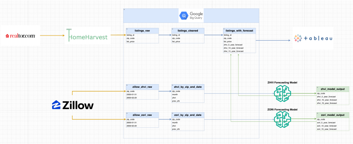
We started by figuring out how to efficiently gather real home listings from a reliable source. Our team utilized HomeHarvest, a Python library that scrapes listings from Realtor.com, to query over 17,000 active listings across the Bay Area over the past 365 days. Each listing includes key information about the property, including list price, location, square footage, etc.. From there, we loaded our script’s raw listings as a table in Google Cloud Platform’s BigQuery and transformed the data to fit the needs of the dashboard by creating a single BigQuery View.
After ingesting our listings data into BigQuery, our next task was to locate home valuation and rental price data over time in order to forecast and surface these metrics to users.
Figure 2: Our data pipeline
Zillow Research provides a handful of free, public datasets related to housing that are updated monthly. One metric that Zillow tracks is the Zillow Home Value Index (ZHVI): “A measure of the typical home value and market changes across a given region and housing type.” We were able to download a dataset that tracks ZHVI per zip code and month since 2000 and load that raw data into BigQuery. From there, we were able to transform and save the raw data into a BigQuery View and create a machine learning Python script that queries the View directly to forecast percentage change in ZHVI (per zip code) in different time horizons (e.g. percentage increase in ZHVI 5 years for zip code 94015). We then pipelined our local machine learning output back to BigQuery and joined the results to our cleaned listings View to forecast a for-sale listing’s home value 5, 10, and 15 years in the future.
Similarly, Zillow has Zillow Observed Rent Index (ZORI): “A smoothed measure of the typical observed market rate rent across a given region.” We created a similar pipeline for a dataset that tracks ZORI per zip code and month to forecast a rental’s projected cost 5, 10 and 15 years in the future.
After joining our forecasting models’ output to our “cleaned” listings View, we ultimately had one “final” View (one row per listing) that we used to fuel our interactive dashboard with important listing features along with our forecasted model output.
3.2.2 Visualization Map
To allow for comparison between buying and renting, the associated cost components that contribute to the total monthly expense of homeownership will be factored to calculate a monthly homeowner cost. As shown by Alcorn, Taryn in "The Hidden Costs of Owning a Home", home ownership often comes with large and unexpected expenses including property taxes, HOA/Condo fees, and maintenance including roof, HVAC, electrical, and plumbing to name a few [10].
Our monthly mortgage payment will assume a fixed-rate mortgage
MP = monthly mortgage payment = (principal * i) / [1 - (1 + i)^-p]
i = monthly interest rate = mortgage rate / 12
p = number of payments = loan term x 12
The final monthly cost for owning a home is calculated as follows:
1) HTMC = Homeowner Total Monthly Cost = MP + TAX + HOA + I + RM + U
TAX = property tax, HOA = monthly HOA/condo fee, I = monthly insurance rate,
RM = monthly repairs/maintenance expense, U = utilities
The final monthly cost for renters is calculated as follows:
2) RTMC = Renters Total Monthly Cost = R + U
R = rent and U = utilities
Implementation Code within Tableau
// Check if status is FOR_RENT or FOR_SALE
IF [Status] = "FOR_RENT" THEN

  // If [List Price] is not null or 0, output [List Price]
  IF [List Price] > 0 THEN
    [List Price]
ELSE
    ([List Price Max] + [List Price Min]) / 2
  END

ELSEIF [Status] = "FOR_SALE" THEN

  // Calculate total monthly cost for home ownership using:
  // Mortgage calculation + HOA Fee
  (([List Price] * [Interest Rate] / 12) / (1 - (1 + [Interest Rate] / 12)^(-[Loan Term (Years)] * 12)))
    + [Hoa Fee] + [Property Tax]*[List Price]/12 + [Repairs and Maintenance %] * [List Price]/12 + [Home Insurance %] * [List Price]/12

ELSE
  NULL // Exclude other statuses
END
3.2.3 Rent Value Percent Change Prediction Model
The data we try to forecast is the percentage of zip-code-level rental change in the next 5, 10, 15 years. To achieve that, the dataset we use to train our models is the average monthly rent of each zip code during the past 20 years (ZORI).
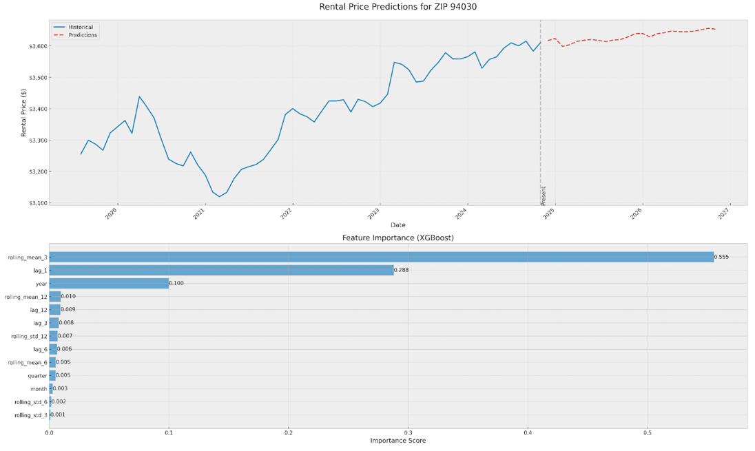
Figure 3: XGBoost_Prophet Model Output
According to Zhang et al, "House rent prediction based on joint model", when it comes to rent prediction, the most commonly seen models are ARIMA, LSTM, XGBoost and Prophet. ARIMA is best for linear, stationary markets with clear trends but limited in handling complex relationships [16]. LSTM excels with large, complex datasets but requires substantial data and computational resources. XGBoost is a robust performer that handles multiple features and non-linear relationships, it has strong predictive power but needs careful feature engineering. Prophet is ideal for seasonal rental markets with built-in trend detection but less flexible with highly irregular data.
As for our model building, for the ARIMA model, auto tuning is used to determine optimal parameters, which is particularly valuable for handling multiple zip codes with different characteristics. This automated approach helps prevent overfitting while ensuring model parameters are optimized for each specific location. LSTM uses a deep learning approach with three stacked layers, the dropout Rate on each layer is 20%. The third model is a weighted combination of XGBoost (60%) and Prophet (40%). Prophet handles trend and seasonality decomposition while XGBoost captures complex feature relationships. Following is the example of the model output:
| zipcode | 5_year_inc (%) | 10_year_inc (%) | 15_year_inc (%) |
|---|---|---|---|
| 94002 | 4.32 | 8.8 | 13.27 |
| 94005 | 4.91 | 9.72 | 14.68 |
| 94010 | 6.36 | 12.87 | 19.38 |
For example, our model forecasts that zip code 94002 will have a 4.32, 8.8 and 13.27 percent increase in ZORI in 5, 10, and 15 years respectively.
3.2.4 Housing Value Percent Change Prediction Model
We aim to forecast the percentage change in home values over the next 5, 10, and 15 years per zip code. Our input data consists of Zillow’s ZHVI for each zip code, spanning from January 2000 to September 2024.
Based on our literature review [5-12], we evaluated several models for this task, including Autoregressive Integrated Moving Average (ARIMA), Long Short-Term Memory (LSTM) networks, and Extreme Gradient Boosting (XGB). The target variable for the input sequences is the ZHVI value of the subsequent month. After fitting the models, one can predict the next month’s ZHVI value given a sequence of past values. To generate forecasts for five years, the prediction process iteratively extends the sequence 60 times—once for each month in the forecast horizon.
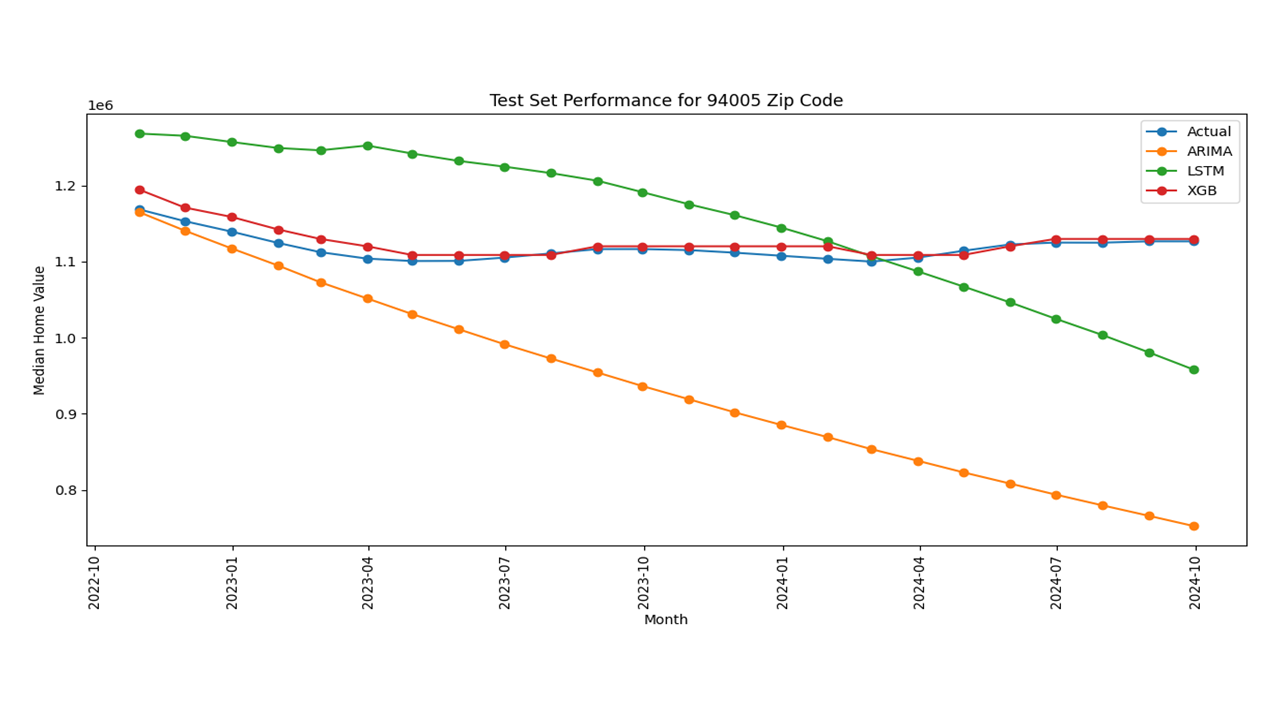
Figures 4-7: Sample Model output for LSTM, XGB, and ARIMA
4. Experiments / Evaluation
Based on our visualization (Figure 1), we can clearly see that the Bay Area is overall a renters’ market with the average calculated monthly cost difference between purchasing and renting is $5,175 (meaning on average a homeowner will spent $5,175 more for their home monthly than a renter in the same zip code).
4.1 User Story 1: Moving to San Francisco
Demo of User Story 1: https://youtu.be/aQb53TiFj4s
“I am moving to San Francisco for a new job out of college. I am looking to rent but don’t know which areas I can get the most bang for my buck over buying. I am open to having a roommate and have a budget of $2,750 a month.”
By filtering on the zip codes for the San Francisco area, we can see which zip codes offer better value from a renter’s perspective compared to purchase costs. In the visualization, we can see that zipcodes in the northwest such as 94121, 94011, and 94114 in gray color are better for renting, over buying. Additionally, we can filter on Cost/Bed to see how much it would cost per bedroom as getting roommates is often a great way to save some money on housing costs.
4.2 User Story 2: Looking to Purchase in Bay Area
Demo of User Story 2: https://youtu.be/XfXWWd4EJ1Y
“I’ve been saving up for many years now and plan to purchase a new house. I currently work remotely and am flexible on location. I would like to know areas where I can get the best value for money compared to renting in the same area.”
By looking at the heatmap alone, we can see the zip codes which the average calculated monthly cost difference between Renting and Owning. We can see that there are only 3 zip (in red color) codes where purchasing is better than renting from a monthly cost perspective (94580, 94939, and 94558). Overall, the Bay Area is heavily skewed in favor of renting over buying.
4.3 Tableau Evaluation and Analysis
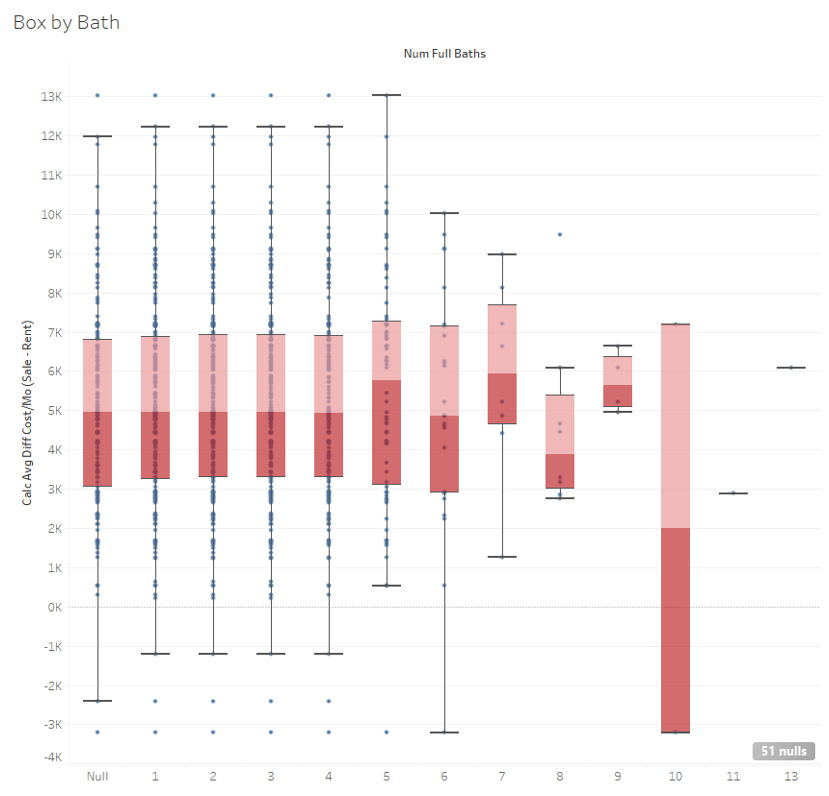
Figure 10: Box Plot by Number of Bathrooms
Observing the Box by Bath Tableau dashboard, shows us that for the number of baths, the dispersion of the calculated monthly cost difference is similar for 1-4 bath listings. We see that for 5 and 6 bath listings, the interquartile spread increases which is to be expected as these typically are more unique listings which can cause increased variation between rentals and for sale total monthly costs. Additionally, as the number of baths increases from 1 to 5, there is a slight increase in favor for renting over buying.
Figure 11: Box Plot by Number of Bedrooms
The Box by Bed Tableau dashboard shows us that 0 bed or studio apartments, 6 beds and above listings, have smaller 1.5x IQR ranges than the 2-5 bed listings which have the greater variation in calculated average difference between sale and rental monthly cost. Translating this for the average consumer, the 2-5 bed listings have greater variation in price difference and thus are potentially opportunities to find a deal depending on the zip code, whether for buying or renting. Conversely, studios and 1 bed listings are more standard and thus there is less price differential for different zip codes between rentals and for sale listings.
4.4 Forecasting Models
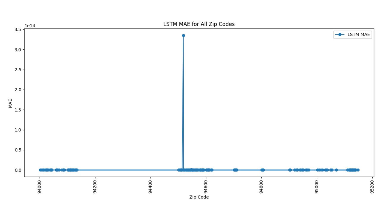
The data set we used to train the models contains almost 25 years of ZHVI data and 10 years of ZORI data for nearly 200 zip codes. For each zip code, we trained each model type on the first 23 years of ZHVI data and 9 years of ZORI data for that zip code, and then made ZHVI predictions for the last 2 years, and ZORI predictions for the final year. We then compared the predictions to the validation set and computed the Mean Absolute Error (MAE) and Mean Absolute Percentage error (MAPE). The table below shows the median MAE/MAPE values across all zip codes for each model type. Median was chosen because there were a few zip codes that generated errors that were extreme outliers. Graphs of the MAE for each model type and zip code can be found in Figures 4-7 and 12-14.
For Sale
| Model | MAE (USD) | MAPE (%) |
|---|---|---|
| LSTM | $292,257.87 | 26.68% |
| ARIMA | $311,772.35 | 25.44 |
| XBG | $16,153.88 | 1.29 |
The XGB model performed the best across both metrics and was chosen as our model to predict home values. The XGB model was roughly $16k off when predicting ZHVI in the test set which was only 1.29% of the home’s value on average.
For Rent
| Model | MAE (USD) | MAPE (%) |
|---|---|---|
| LSTM | $64.53 | 1.73% |
| ARIMA | $67.89 | 1.82 |
| XBG | $51.36 | 1.37 |
Based on the metrics, the combined XGBoost_Prophet model is chosen as our rent forecast model. It was roughly $51.36 off when predicting ZORI in the test set which was only 1.37% off the monthly rent on average.
Figures 12-14: Model Evaluation
5. Conclusions & Discussion
Our project showcases the power of integrating data pipelines with advanced forecasting models. By leveraging Google’s cloud-based platform, BigQuery, and a Python-based machine learning framework, we were able to construct a scalable data pipeline that efficiently gathered and processed housing data. The resulting pipeline allows for real-time updates and future scalability, supporting dynamic housing market analysis and predictive insights.
The forecast model evaluation highlights the effectiveness of combining multiple machine learning techniques to forecast housing and rental trends. Each of the models tested had their strengths, but the XGBoost-Prophet hybrid model outperformed other models, achieving the lowest MAE and the lowest MAPE. This underlines the importance of using composite models for capturing the intricacies of housing data, including non-linear trends and seasonality, which simple models often miss.
Our visualization component, built in Tableau, was essential for making the data easy to use and actionable for users. By allowing users to explore housing affordability through interactive dashboards, we were able to bridge the gap between data complexity and user comprehension. The dashboard's filtering and customization capabilities and the breakdown of homeowner and renter costs empower users to make informed decisions tailored to their personal financial circumstances.
Despite these successes, limitations remain. While the model performed well in evaluating past trends, future improvements could include expanding beyond the Bay Area and incorporating additional external data such as crime, economic indicators, and/or social indicators as those discussed in the literature [4-7]. Additionally, while the model incorporates hyperparameter tuning, further fine-tuning could improve predictive accuracy for individual zip codes with unique market dynamics. Finally, it’s important to consider not all houses are created equally and that all models can only attempt to find patterns in housing value.
In conclusion, our approach to comparing renting and buying with advanced forecasting tools provides a substantial improvement over existing market tools. By making complex data more transparent and accessible, we have created a foundational framework for a tool that can be further developed to support more informed housing decisions for a diverse range of users.
6. Sources & Citations
Data Sources
Zillow. "Housing Data." Zillow Research, https://www.zillow.com/research/data/. Accessed 10/20/2024.
Bunsly. "HomeHarvest: A Python Package for Real Estate Data Analysis." GitHub, https://github.com/Bunsly/HomeHarvest. Accessed 10/11/2024.
Research Papers
[1] Oxford Economics. (n.d.). Housing has become less affordable across all US metros. Retrieved November 18, 2024, from https://www.oxfordeconomics.com/resource/housing-has-become-less-affordable-across-all-us-metros/
[2] Norada Real Estate Investments. (2024, October 31). San Francisco real estate market: Trends and analysis for 2024. Retrieved November 19, 2024, from https://www.noradarealestate.com/blog/san-francisco-real-estate-market/
[3] Sundar, S. S., & Kalyanaraman, S. (2020). The impact of media on public opinion: An analysis of framing and salience in political discourse. Political Psychology, 31(1), 30–50. https://doi.org/10.1093/ppar/pzz011
[4] Styhre, A., Brorström, S., & Gluch, P. (2022). The valuation of housing in low-amenity and low purchasing power city districts: social and economic value entangled by default. Construction Management and Economics, 40(1), 72–86. https://doi.org/10.1080/01446193.2021.2018719
[5] Aizenman, J., Jinjarak, Y., & Zheng, H. (2016). House Valuations and Economic Growth: Some International Evidence (NBER Working Paper No. 22699). National Bureau of Economic Research. https://doi.org/10.3386/w22699
[6] Numan, Jamal A. A., and Izham Mohamad Yusoff. "Identifying the Current Status of Real Estate Appraisal Methods." Real Estate Management and Valuation, vol. 32, no. 1, 2024, pp. 1-15. https://doi.org/10.2478/remav-2024-0032
[7] Alcorn, Taryn. "The Hidden Costs of Owning a Home." Investopedia, 12 Apr. 2023, www.investopedia.com/the-hidden-costs-of-owning-a-home-4776306.
[8] Benidis, Konstantinos, et al. "Deep learning for time series forecasting: Tutorial and literature survey." ACM Computing Surveys 55.6 (2022): 1-36.
[9] Paliari, Iliana, Aikaterini Karanikola, and Sotiris Kotsiantis. "A comparison of the optimized LSTM, XGBOOST and ARIMA in Time Series forecasting." 2021 12th International Conference on Information, Intelligence, Systems & Applications (IISA). IEEE, 2021.
[10] Joseph, LMI Leo, et al. "Predicting Real-Time House Prices: A Machine Learning Approach Using XGBoost Algorithm." 2024 Asia Pacific Conference on Innovation in Technology (APCIT). IEEE, 2024.
[11] Jadevicius, Arvydas, and Simon Huston. "ARIMA modelling of Lithuanian house price index." International Journal of Housing Markets and Analysis 8.1 (2015): 135-147.
[12] Liu, Jun, and Zihan Ma. "Forecasting Housing Price Using GRU, LSTM and Bi-LSTM for California." 2024 IEEE 2nd International Conference on Control, Electronics and Computer Technology (ICCECT). IEEE, 2024.
[Paper 13] Ziyadi, Hossein, Erfan Salavati, and Mohammad Mahdi Lotfi Heravi. "Housing Price Forecasting Using AI (LSTM)." Financial Research Journal 25.4 (2023): 557-576.
[Paper 14] Mach, Łukasz, et al. "The Identification of Seasonality in the Housing Market Using the X13-ARIMA-SEATS Model." Econometrics 27.4 (2023): 29-43.
[Paper 15] Hjort, Anders, et al. "House price prediction with gradient boosted trees under different loss functions." Journal of Property Research 39.4 (2022): 338-364.
[Paper 16] Zhang, Kun, LingCong Shen, and Ningning Liu. "House rent prediction based on joint model." Proceedings of the 2019 8th International Conference on Computing and Pattern Recognition. 2019.
Special thanks to my project teammates, James Marvin, Qing Yu, and Tyler Chang for their contributions and hard work all semester and best of luck!


